ABC Example#
In this tutorial we’ll measure spot properties for the FGK stars in Praesepe by
approximating the light curve smoothed amplitude distribution using Approximate
Bayesian Computation (ABC).
We’ll use astroquery to download the pre-calculated light curve smoothed amplitudes from
Douglas et al. (2017).
We’ll compute the two-sample Anderson-Darling statistic
as a summary statistic to measure whether how close the simulated light curve
amplitude distribution is to the observed distribution of smoothed amplitudes,
and accept steps in the chain that have small A-D statistics.
First let’s import tools the standard Python science stack, plus astroquery
and corner:
import matplotlib.pyplot as plt
import numpy as np
from scipy.stats import anderson_ksamp
import astropy.units as u
from astroquery.vizier import Vizier
from corner import corner

from fleck import generate_spots, Star
Let’s use astroquery to retrieve the smoothed amplitudes of Praesepe FGK
stars:
Vizier.ROW_LIMIT = -1

v = Vizier(catalog='J/ApJ/842/83/table3', columns=["**"], row_limit=-1)
table = v.query_constraints()[0]

fgk_stars = (~table['SmAmp'].mask) & (table['Mass'] > 0.6 * u.Msun)
amplitudes_praesepe = 2 * table['SmAmp'][fgk_stars].data
We must multiply the reported smoothed amplitudes by a factor of two as they were recorded as semi-amplitudes by Douglas et al. (2017).
Let’s set up our stellar sample properties, and prepare to measure 100 randomly distributed stellar inclinations at each realization of the simulation:
# quadratic limb darkening parameters
ld = [0.5079, 0.2239]
# Evaluate the model 30 times per rotation, set fiducial spot parameters
stars = Star(spot_contrast=0.7, n_phases=30, u_ld=ld)
n_inclinations = 100
spot_radius = 0.2
# Fix the number of spots on the star to three:
n_spots = 3
We must also define the summary statistic which compares the simulated light curve amplitude distribution to the observed one, for a given set of spot parameters:
def ad(spot_radius, max_latitude, spot_contrast):
    stars.spot_contrast = spot_contrast
    lons, lats, rads, incs = generate_spots(min_latitude=-max_latitude,
                                            max_latitude=max_latitude,
                                            n_spots=n_spots,
                                            spot_radius=spot_radius,
                                            n_inclinations=n_inclinations)
    lcs = stars.light_curve(lons, lats, rads, incs)

    # Convert light curves to smoothed amplitudes (%):
    smoothed_amps = 100 * lcs.ptp(axis=0)

    # Compute the Anderson-Darling statistic between the two samples in
    # log space:
    anderson_stat = anderson_ksamp([np.log10(smoothed_amps),
                                    np.log10(amplitudes_praesepe)]).statistic
    return anderson_stat
Finally we set up the chains and a while loop that will iterate until the
number of required step have been added to the chain:
# Number of successful steps to iterate over
n_steps = 5000

# Initial spot parameters
init_rad = 0.23
init_max_lat = 70
init_contrast = 0.7

# Initialize chains with init step
ad_stats = [ad(init_rad, init_max_lat, init_contrast)]
spot_radii = [init_rad]
max_lats = [init_max_lat]
spot_contrasts = [init_contrast]
steps = 0
accepted_step = 0

while accepted_step < n_steps:
    spot_radius = 0.05 * np.random.randn() + spot_radii[accepted_step]
    max_lat = 5 * np.random.randn() + max_lats[accepted_step]
    spot_contrast = 0.1 * np.random.randn() + spot_contrasts[accepted_step]

    # Apply prior
    if 0 < spot_radius < 1 and 0 < max_lat < 90 and 0 < spot_contrast < 1:
        adstat = ad(spot_radius, max_lat, spot_contrast)

        steps += 1

        # If summary statistic is less than threshold:
        if adstat < 0:
            # Accept step
            spot_radii.append(spot_radius)
            max_lats.append(max_lat)
            spot_contrasts.append(spot_contrast)
            ad_stats.append(adstat)
            accepted_step += 1
We can visualize the results by making a corner plot:
fig, ax = plt.subplots(3, 3, figsize=(5, 5))
samples = np.array([max_lats, spot_radii, spot_contrasts]).T
corner(samples, labels='$\\rm\ell_{max}$ $\\rmR_{spot}/R_{star}$ $c$'.split(),
       smooth=True, fig=fig);
plt.show()
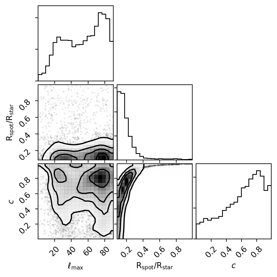
The corner plot shows us the posterior distributions for the three spot parameters: the maximum spot latitude \(\ell_{max}\), the spot radius \(\rm R_{spot}/R_{star}\), and the spot contrast \(c\). As we might expect, \(\rm R_{spot}/R_{star}\) is degenerate with \(c\): large spots with small contrasts can be swapped for smaller spots with higher contrasts and produce equally good approximations to the smoothed amplitude distribution of Praesepe stars.