MCMC Example#
In this tutorial, we’ll fit the light curve of the 23 ± 4 Myr-old transiting
exoplanet star V1298 Tau with fleck.
It is interesting to apply fleck to V1298 Tau because it is young and
spotted, and has repeated spot signals over the duration of a few stellar
rotations. Here, we’ll use lightkurve to download the K2 photometry,
astropy to measure the stellar rotation period with a Lomb-Scargle,
periodogram, and finally fleck to model the rotational modulation of the
host star in order to invert the light curve for the spot properties: latitudes,
longitudes, and radii.
First, we import all of the required packages for this tutorial:
import matplotlib.pyplot as plt
import numpy as np
from astropy.coordinates import SkyCoord
from astropy.timeseries import LombScargle
import astropy.units as u
import healpy as hp
from lightkurve import search_lightcurve
from emcee import EnsembleSampler
from multiprocessing import Pool
from corner import corner
from fleck import Star
Note
These examples require a few extra dependencies, get them with:
pip install fleck[docs]
Next we resolve the target coordinates using astropy, and download its light
curve using lightkurve’s handy method:
coord = SkyCoord.from_name('V1298 Tau')
slcf = search_lightcurve(coord, mission='K2')

lc = slcf.download_all()
pdcsap = lc.PDCSAP_FLUX.stitch()

time = pdcsap.time
flux = pdcsap.flux

notnanflux = ~np.isnan(flux)

flux = flux[notnanflux & (time > 2230) & (time < 2239)]
time = time[notnanflux & (time > 2230) & (time < 2239)]

flux /= np.mean(flux)
Next, we want to determine the stellar rotation period, which will remain fixed
in our fleck analysis. We do this with a Lomb-Scargle periodogram:
periods = np.linspace(1, 5, 1000) * u.day
freqs = 1 / periods
powers = LombScargle(time * u.day, flux).power(freqs)
best_period = periods[powers.argmax()]
Now that we know that the best period is roughly 2.87 days, we can generate
fleck light curves that reproduce the spot modulation:
u_ld = [0.46, 0.11]
contrast = 0.7
phases = (time % best_period.value) / best_period.value
s = Star(contrast, u_ld, n_phases=len(time), rotation_period=best_period.value)

init_lons = np.array([0, 320, 100])
init_lats = [0, 20, 0]
init_rads = [0.01, 0.2, 0.3]

yerr = 0.002

init_p = np.concatenate([init_lons, init_lats, init_rads])
With our initial parameters set, we now define the functions that emcee uses
to do Markov Chain Monte Carlo:
def log_likelihood(p):
    lons = p[0:3]
    lats = p[3:6]
    rads = p[6:9]

    lc = s.light_curve(lons[:, None] * u.deg, lats[:, None] * u.deg, rads[:, None],
                       inc_stellar=90*u.deg, times=time, time_ref=0)[:, 0]

    return - 0.5 * np.sum((lc/np.mean(lc) - flux)**2 / yerr**2)

def log_prior(p):
    lons = p[0:3]
    lats = p[3:6]
    rads = p[6:9]

    if (np.all(rads < 1.) and np.all(rads > 0) and np.all(lats > -60) and
        np.all(lats < 60) and np.all(lons > 0) and np.all(lons < 360)):
        return 0
    return -np.inf

def log_probability(p):
    lp = log_prior(p)
    if not np.isfinite(lp):
        return -np.inf
    return lp + log_likelihood(p)
We’ll run the chains for a short period of time to see the results faster, but to ensure convergence, you should run for 10-100x longer than this example:
ndim = len(init_p)
nwalkers = 5 * ndim
nsteps = 5000

pos = []


while len(pos) < nwalkers:
    trial = init_p + 0.01 * np.random.randn(ndim)
    lp = log_prior(trial)
    if np.isfinite(lp):
        pos.append(trial)

with Pool() as pool:
    sampler = EnsembleSampler(nwalkers, ndim, log_probability, pool=pool)
    sampler.run_mcmc(pos, nsteps, progress=True);

samples_burned_in = sampler.flatchain[len(sampler.flatchain)//2:, :]
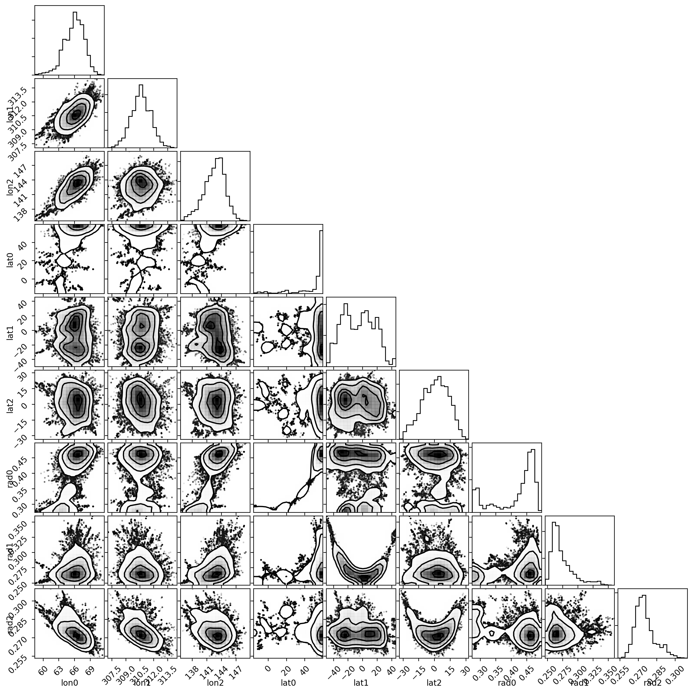
Now let’s plot the corner plot with the posterior distributions and their
correlations using the corner package:
fig, ax = plt.subplots(9, 9, figsize=(12, 12))
labels = "lon0 lon1 lon2 lat0 lat1 lat2 rad0 rad1 rad2".split()
corner(samples_burned_in, smooth=True, labels=labels,
       fig=fig);
plt.show()
Finally, let’s plot several draws from the posterior distributions for near the
maximum-likelihood light curve model, the total spot coverage posterior
distribution, and the spot map using healpy:
fig, ax = plt.subplots(1, 3, figsize=(8, 1.5))

for i in np.random.randint(0, len(samples_burned_in), size=50):

    trial = samples_burned_in[i, :]

    lons = trial[0:3]
    lats = trial[3:6]
    rads = trial[6:9]

    lc = s.light_curve(lons[:, None] * u.deg, lats[:, None] * u.deg, rads[:, None],
                       inc_stellar=90*u.deg, times=time, time_ref=0)[:, 0]
    ax[0].plot(time, lc/lc.mean(), color='DodgerBlue', alpha=0.05)

f_S = np.sum(samples_burned_in[:, -3:]**2 / 4, axis=1)

ax[1].hist(f_S, bins=25, histtype='step', lw=2, color='k', range=[0, 0.12], density=True)
ax[0].set(xlabel='BJD - 2454833', ylabel='Flux', xticks=[2230, 2233, 2236, 2239])
ax[1].set_xlabel('$f_S$')
ax[0].plot(time, flux, '.', ms=2, color='k', zorder=10)

NSIDE = 2**10

NPIX = hp.nside2npix(NSIDE)

m = np.zeros(NPIX)

np.random.seed(0)
random_index = np.random.randint(samples_burned_in.shape[0]//2,
                                 samples_burned_in.shape[0])
random_sample = samples_burned_in[random_index].reshape((3, 3)).T
for lon, lat, rad in random_sample:
    t = np.radians(lat + 90)
    p = np.radians(lon)
    spot_vec = hp.ang2vec(t, p)
    ipix_spots = hp.query_disc(nside=NSIDE, vec=spot_vec, radius=rad)
    m[ipix_spots] = 0.7

cmap = plt.cm.Greys
cmap.set_under('w')

plt.axes(ax[2])
hp.mollview(m, cbar=False, title="", cmap=cmap, hold=True,
            max=1.0, notext=True, flip='geo')
hp.graticule(color='silver')

fig.suptitle('V1298 Tau')

for axis in ax:
    for sp in ['right', 'top']:
        axis.spines[sp].set_visible(False)
plt.show()
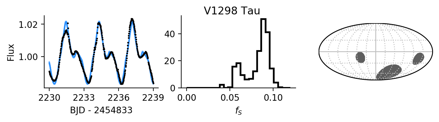
Finally, we can print the spot coverage:
lo, mid, hi = np.percentile(f_S, [16, 50, 84])
print(f"$f_S = {{{mid:g}}}^{{+{hi-mid:g}}}_{{-{mid-lo:g}}}$")
which returns \(f_S = {0.087}^{+0.006}_{-0.025}\).