Differential Rotation

fleck can be used to generate light curves of stars with spots and differential rotation. To start, we import fleck, and create two helper functions:

import matplotlib.pyplot as plt
import numpy as np
import astropy.units as u

from fleck import Star, generate_spots


def solar_diff_rot(latitude, scale_factor=1):
    """
    Use simple approximate the solar differential rotation profile from
    Howard et al. (1984) to return the rotation period of spots
    distributed at ``latitude``. Scale up (or down) the magnitude
    of stellar differential rotation by factor ``scale_factor``.

    Parameters
    ----------
    latitude : `~astropy.units.Quantity`
        Latitudes of spots
    scale_factor : float
        Stretch the differential rotation profile by
        a constant factor

    Returns
    -------
    prots : `~numpy.ndarray`
        Rotation period for each spot ``latitude``
    """
    omega = scale_factor * (14.522 - 2.840 *
                            np.sin(latitude)**2) * u.deg / u.day
    return (2*np.pi / omega).to(u.day/u.rad).value[0]

def interpolate_phase_to_time(times, phases, prots, lcs):
    """
    Linearly interpolate individual spot light curves ``lcs``
    evaluated at ``phases`` on the new time grid ``times``

    Parameters
    ----------
    times : `~numpy.ndarray`
        Time axis to interpolate onto
    phases : `~astropy.units.Quantity`
        Original phase axis on which ``lcs`` was computed
    prots : `numpy.ndarray`
        Rotation period array, one per spot
    lcs : `~numpy.ndarray`
        Individual spot light curves

    Returns
    -------
    interp_lcs : `~numpy.ndarray`
        Interpolated light curves evaluated at ``times``
    """
    f = np.zeros((len(times), len(prots)))

    for i, prot in enumerate(prots):
        f[:, i] = np.interp(times,
                            phases.value * prot / (2*np.pi),
                            lcs[:, i])

    return f

With these two functions defined, we’re ready to begin generating light curves. First let’s initialize a bunch of light curves as though we were using fleck normally, except this time the n_spots argument will be fixed to 1, and the multiple (identical) stellar inclinations computed will be used to compute the effect of spots at different latitudes rotating with different rotation periods:

# Make plots reproducible
np.random.seed(42)

# Set spot contrast, limb-darkening parameters
spot_contrast = 0.7
u_ld = [0.5079, 0.2239]

# The phase axis on which fleck will evaluate the light curves
# will be defined on [0, `max_phase`]:
max_phase = 1250
phases = np.linspace(0, max_phase, 10 * max_phase) * u.rad

# The time axis on which the final light curve will be evaluated
# is some fraction `interp_fraction` of the span of the initial
# phase axis
interp_fraction = 0.8
times = np.linspace(0, int(interp_fraction * max_phase),
                    int(interp_fraction * 0.5 * max_phase))

# Generate `n_spots` spots distributed
# between `min_latitude` and `max_latitude`, with size
# `spot_radius` for a star viewed at `stellar_inclination`
# where 90 deg = equator-on, 0 deg = pole-on.
n_spots = 2
spot_radius = 0.1         # Rspot/Rstar
min_latitude = 15         # deg
max_latitude = 30         # deg
stellar_inclination = 90  # deg

inclinations = stellar_inclination * u.deg * np.ones(n_spots)
lons, lats, radii, inc_stellar = generate_spots(min_latitude, max_latitude,
                                                spot_radius, n_spots=1,
                                                inclinations=inclinations)

star = Star(spot_contrast=spot_contrast, phases=phases, u_ld=u_ld)
lcs = star.light_curve(lons, lats, radii, inc_stellar)

Now lcs contains the individual spot contributions to a light curve, with shape (12500, 2) – the first axis represents the number of phases at which we computed the light curves, and the second axis is the number of spots.

We can now assign different rotation periods for each spot by evaluating the (solar) differential rotation shear at each latitude and interpolating the resulting light curves onto the same time axis:

solar_diff_rot_factor = 1  # Scale up/down solar differential rotation

# To add differential rotation, interpolate rotation curves
# as function of phase onto a time axis:
prots = solar_diff_rot(lats, scale_factor=solar_diff_rot_factor)
interp_lcs = interpolate_phase_to_time(times, phases, prots, lcs)

# The differential rotation light curve is the sum of the
# light curves along the 1st axis.
dr_lc = interp_lcs.sum(axis=1) / interp_lcs.shape[1]

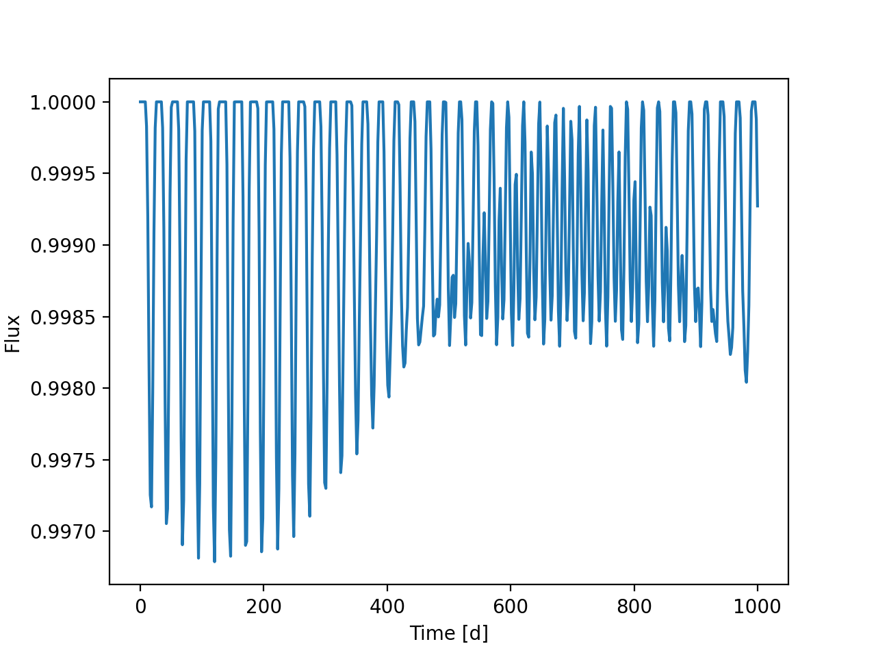
Finally we can plot the result:

plt.plot(times, dr_lc)

plt.gca().set(xlabel='Time [d]',
              ylabel='Flux')

(Source code, png, hires.png, pdf, svg)

Notice that the resulting light curve has some complex morphology that could easily be mistaken for spot evolution.