JAX Interface#
Warning
If you install fleck via pip, you may not have the jax
dependencies necessary for this module. To ensure that you do,
follow the instructions for jax compatibility in Installation.
Intro#
We’re going to compute the transmission spectrum for a transit of TRAPPIST-1 c, assuming the planet has no atmosphere and the transmission spectrum changes with wavelength due only to stellar surface features. We will place one warm and one cool active region on the photosphere,
Note
This tutorial depends on the package expecto
(code,
docs). You can
install expecto via pip with:
python -m pip install expecto
First, we need to import some things,
import matplotlib.pyplot as plt
from matplotlib.gridspec import GridSpec

import numpy as np
import astropy.units as u
from expecto import get_spectrum

from jax import numpy as jnp
from fleck.jax import ActiveStar, bin_spectrum
and we choose the times and wavelengths at which to compute the spectrophotometry for our active star+planet model,
times = np.linspace(-0.04, 0.04, 250)
wavelength = np.geomspace(0.5, 5, 101) * u.um
Choose active region spectra#
Active regions emit spectra that are distinct from the photosphere.
In this model, we will use three PHOENIX model spectra, downloaded
via the expecto package.
The photospheric, cool, and warm regions will have temperatures:
\(T_{\rm phot}=2600 {\rm ~K}\),
\(T_{\rm cool}=2400 {\rm ~K}\), and
\(T_{\rm warm}=2800 {\rm ~K}\), all with the same surface gravity.
We will bin those spectra onto the wavelength grid that we chose
above using bin_spectrum:
# Set model spectrum binning preferences:
kwargs = dict(
    bins=wavelength,
    min=wavelength.min(),
    max=wavelength.max(),
    log=False
)

# Download and bin PHOENIX model spectra:
phot, cool, hot = [
    bin_spectrum(
        get_spectrum(T_eff=T_eff, log_g=5.0, cache=True), **kwargs
    )
    for T_eff in [2600, 2400, 2800]
]
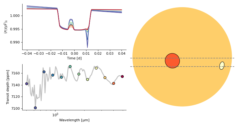
We will visualize the contaminated transmission spectrum, the transit light curves at several wavelengths, and a 2D orthographic projection of the stellar surface. A lot of code goes into making such a plot, which we have hidden in this collapsible element in the documentation below. If you’re interested in how it works, click it to expand.
Construct a model for an active star#
Now we define our ActiveStar model by the specific times and wavelengths
that we will observe, the stellar inclination, and spectrum of the stellar photosphere.
# stellar parameters:
active_star = ActiveStar(
    times=times,
    inclination=np.pi/2,  # stellar inc [rad]
    T_eff=phot.meta['PHXTEFF'],
    wavelength=phot.wavelength.to_value(u.m),
    phot=phot.flux.value,
)
We can add active regions to the star with add_spot
# add a cool spot:
active_star.add_spot(
    lon=-0.2,  # [rad]
    lat=1.65,  # [rad]
    rad=0.15,  # [R_star]
    spectrum=cool.flux.value,
    temperature=cool.meta['PHXTEFF']
)

# add a hot spot:
active_star.add_spot(
    lon=0.95,
    lat=1.75,
    rad=0.08,
    spectrum=hot.flux.value,
    temperature=hot.meta['PHXTEFF']
)
Add a transiting planet with spot occultations#
In order to model the transit of a planet, we need to define the planet’s parameters like so:
# planet parameters for TRAPPIST-1 c from Agol 2021:
t1c = dict(
    inclination = np.radians(89.778),
    a = 28.549,
    rp = 0.08440,
    period = 2.421937,
    t0 = 0,
    ecc = 0,
    u1 = 0.1,
    u2 = 0.3
)
And finally, we’re prepared to make the plot. We will call the function
plot_transit_contamination below, which we defined in a collapsible
code cell above, makes a lot of plotting calls to visualize the results of
transit_model and
plot_star:
plot_transit_contamination(active_star, t1c)
(Source code, png, hires.png, pdf, svg)

In the plot above, several time series light curves are shown in the top left, where each color corresponds to a different wavelength. There is an occultation of the cool spot by the planet just before mid-transit, and an occultation of the hot spot by the planet just before egress. Rotational modulation of the star is seen in the slope in the wavelength dependent out-of-transit flux.
The plot in the bottom left shows the apparent transmission spectrum as the planet
transits the star. For an airless planet with rp = 0.08440, the expected transit
depth (rp**2) is 7123 ppm, and the deviations from that value in the transmission
spectrum arise from unocculted active regions. The colored points on the spectrum
label the wavelengths of each light curve of the same color on the upper left panel.
The stellar schematic on the right shows the stellar surface with the photosphere in light orange, the cool region with darker orange, and the warm region in light yellow. The two dashed lines trace the upper and lower limit of the planet’s transit chord. The transit occurs with ingress on the left of the plot, and egress to the right, and the stellar rotation occurs in the same direction.