Getting started

Rotational modulation

Suppose you want to observe 100 stars with randomly drawn stellar inclinations, each with spot contrast c=0.7 (where c=0 means perfectly dark spots), with quadratic limb-darkening. Let’s distribute three spots on each star randomly above 70 degrees latitude up to the pole. We can use the generate_spots method to quickly create spot property matrices in the correct shape:

from fleck import generate_spots

spot_contrast = 0.7
u_ld = [0.5079, 0.2239]

n_phases = 30
n_inclinations = 100
n_spots = 3

spot_radius = 0.1   # Rspot/Rstar
min_latitude = 70   # deg
max_latitude = 90   # deg

lons, lats, radii, inc_stellar = generate_spots(min_latitude, max_latitude,
                                                spot_radius, n_spots,
                                                n_inclinations=n_inclinations)

lons, lats, radii will each have shape (n_spots, n_inclinations) and inc_stellar will have shape (n_inclinations, ). Now let’s initialize a Star object:

from fleck import Star

star = Star(spot_contrast=spot_contrast, n_phases=n_phases, u_ld=u_ld)

If we initialize the Star object with a number of phases n_phases, it will evenly sample all phases on \((0, 2\pi)\).

Now we can compute light curves for stars with the spots we generated like so:

lcs = star.light_curve(lons, lats, radii, inc_stellar)

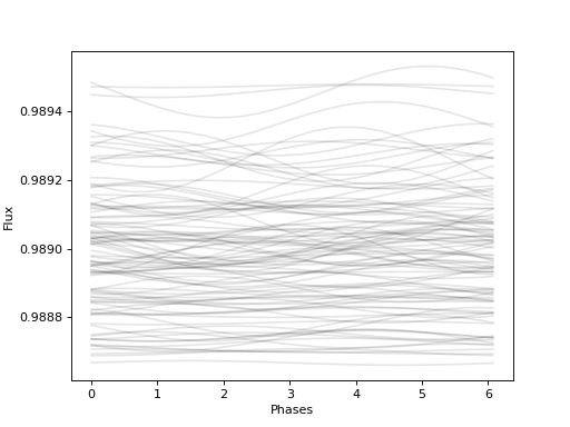
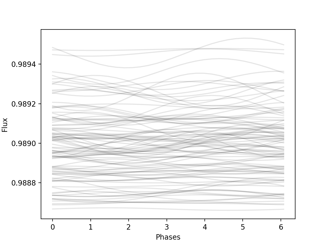
where lcs will have shape (n_phases, n_inclinations). Let’s plot each of the light curves:

import matplotlib.pyplot as plt
plt.plot(star.phases, lcs)
plt.show()

(Source code, png, hires.png, pdf, svg)

Spot Occultations

Now let’s make a transiting exoplanet, and observe spot occultations. We can specify the parameters of the transiting exoplanet using the same specification used by batman:

from batman import TransitParams
import astropy.units as u

planet = TransitParams()
planet.per = 88
planet.a = float(0.387*u.AU / u.R_sun)
planet.rp = 0.1
planet.w = 90
planet.ecc = 0
planet.inc = 90
planet.t0 = 0
planet.limb_dark = 'quadratic'
planet.u = [0.5079, 0.2239]

Let’s now specify some spots on the stellar surface:

import numpy as np

inc_stellar = 90 * u.deg
spot_radii = np.array([[0.1], [0.1]])
spot_lats = np.array([[0], [0]]) * u.deg
spot_lons = np.array([[360-30], [30]]) * u.deg

and some times at which to observe the system:

times = np.linspace(-0.5, 0.5, 500)

let’s initialize our Star object, specifying a stellar rotation period:

from fleck import Star
star = Star(spot_contrast=0.7, u_ld=planet.u, rotation_period=10)

We generate a light curve using the same light_curve method that we used earlier, but this time we will supply it with the planet’s parameters and the times at which to evaluate the model:

lc = star.light_curve(spot_lons, spot_lats, spot_radii,
                      inc_stellar, planet=planet, times=times)

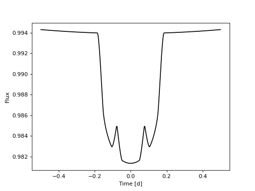
Finally we can plot the transit light curve:

import matplotlib.pyplot as plt
plt.plot(times, lc, color='k')
plt.show()

(Source code, png, hires.png, pdf, svg)

Plotting

You can make quick plots for debugging and understanding a system’s geometry using the plot method. For example, let’s create a star observed at an odd angle, with a misaligned planet:

from batman import TransitParams
import matplotlib.pyplot as plt
import numpy as np
import astropy.units as u
from fleck import Star

planet = TransitParams()
planet.per = 88
planet.a = float(0.387*u.AU / u.R_sun)
planet.rp = 0.1
planet.w = 90
planet.ecc = 0
planet.inc = 89.65
planet.t0 = 0
planet.limb_dark = 'quadratic'
planet.u = [0.5079, 0.2239]

We define the angular offset between the planet’s orbit normal and the spin the star projected onto the sky plane (often denoted \(\lambda\)) using the extra planet parameter planet.lam, in units of degrees:

planet.lam = 45

The stellar inclination (measured away from the sub-observer point) often denoted \(i_s\) is defined:

inc_stellar = 70 * u.deg

Let’s create two spots along one line of longitude:

spot_radii = np.array([[0.1], [0.1]])
spot_lons = np.array([[0], [0]]) * u.deg
spot_lats = np.array([[25], [-25]]) * u.deg

Let’s now observe the system:

times = np.linspace(-0.5, 0.5, 500)

star = Star(spot_contrast=0.7, u_ld=planet.u, rotation_period=10)
ax = star.plot(spot_lons, spot_lats, spot_radii, inc_stellar, planet=planet,
               time=0)

plt.show()

(Source code, png, hires.png, pdf, svg)

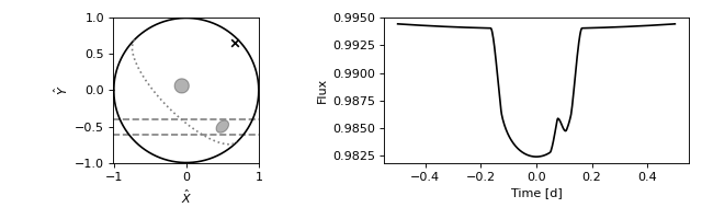
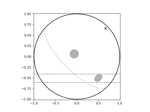
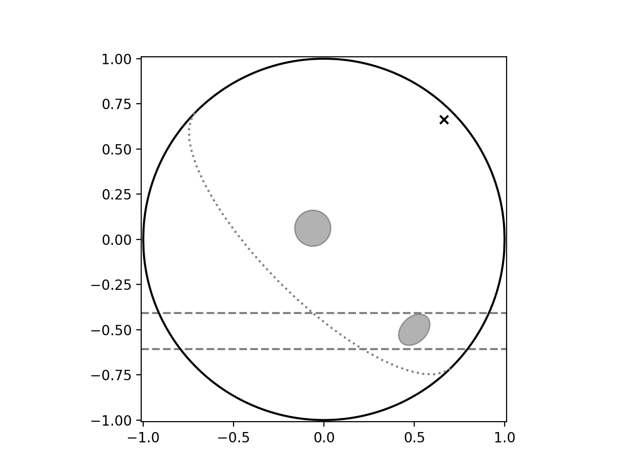
The black x marks the location of the stellar rotational pole. Gray ellipses mark each starspot. The horizontal gray dashed lines represent the upper and lower bounds of the exoplanet’s transit chord over the star. The planet transits from left to right across this coordinate system. The stellar equator is marked with a dotted gray line.

We can plot the transit light curve and the system geometry on the same figure like so:

(Source code, png, hires.png, pdf, svg)